When I learnt about free software some time ago, I came to believe that software patents were a very insidious threat. It was dangerous that someone could claim exclusivity over an algorithm: it could stifle innovation, it could be an obstacle to independent free software implementations of useful standards, etc. I very much hoped that Europe would keep them at bay, and still remember when the corresponding directive was rejected in 2005, giving us the relative security that we now enjoy in the EU in comparison with other countries such as the USA.

Since then, some of my work about speech recognition while interning at Google New York has been turned into a US patent application that was recently published. I was paid a patent bonus by Google and assisted them to fix problems in drafts of the application. This process has given me more elements to form an opinion about software patents in the US, and I have changed my mind accordingly. I no longer believe that they are an insidious threat. I now believe them to be a blatant absurdity.

I invite anyone doubting this fact to skim through the application and see for themselves. Just for fun, here are some selected bits.

Our tour begins with a wall of boilerplate on pages 2 to 4 that describes mundane banalities about computers in a stilted prose that makes a surreal attempt at complete and exhaustive generality. (Remember that the topic is speech recognition, with printers and light bulbs being key components of such systems, as we all know.)

[0058] User interface 304 may function to allow client device 300 to interact with a human or non-human user, such as to receive input from a user and to provide output to the user. Thus, user interface 304 may include input components such as a keypad, keyboard, touch-sensitive or presence-sensitive panel, computer mouse, trackball, joystick, microphone, still camera and/or video camera. User interface 304 may also include one or more output components such as a display screen (which, for example, may be combined with a presence-sensitive panel), CRT, LCD, LED, a display using DLP technology, printer, light bulb, and/or other similar devices, now known or later developed. User interface 304 may also be configured to generate audible output(s), via a speaker, speaker jack, audio output port, audio output device, earphones, and/or other similar devices, now known or later developed. In some embodiments, user interface 304 may include software, circuitry, or another form of logic that can transmit data to and/or receive data from external user input/output devices. Additionally or alternatively, client device 300 may support remote access from another device, via communication interface 302 or via another physical interface (not shown).

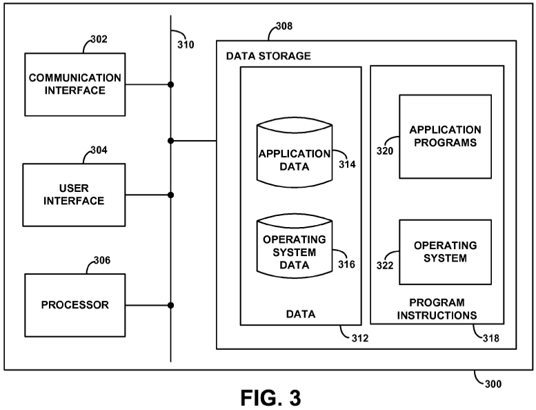
It seems that you have to describe the overall context of the invention from scratch, even though it implies you have to repeat the same platitudes in every single application. In case you are wondering about those numbers peppered throughout, they are actually pointers to a helpful figure that wouldn't look out of place in a 1990 monograph about computer architecture:

Let us now move on to the gruesome sight of mathematical language being contorted and twisted to fit this strange mode of expression. The bulk of the application reads like a scientific paper eerily addressed to lawyers from the past. Here is an example from page 11:

[0162] As noted above, the search graph may be prepared by pushing the weights associated with some transitions toward the initial state such that the total weight of each path is unchanged. In some embodiments, this operation provides that for every state, the sum of all outgoing edges (including the final weight, which can be seen as an E-transition to a super-final state) is equal to 1.

Confused? Here is the beginning of the conclusion, that wraps things up in a surprisingly inconclusive way. I think the point is to make a desperate appeal to the reader to use their common sense, but I'm not sure.

[0192] The above detailed description describes various features and functions of the disclosed systems, devices, and methods with reference to the accompanying figures. In the figures, similar symbols typically identify similar components, unless context indicates otherwise. The illustrative embodiments described in the detailed description, figures, and claims are not meant to be limiting. Other embodiments can be utilized, and other changes can be made, without departing from the spirit or scope of the subject matter presented herein. It will be readily understood that the aspects of the present disclosure, as generally described herein, and illustrated in the figures, can be arranged, substituted, combined, separated, and designed in a wide variety of different configurations, all of which are explicitly contemplated herein.

The forced marriage between legalese and theoretical computer science jargon reaches its peak in the claim list. Reproducing it in full here would be both inconvenient and intolerable, but here is the general flavor:

An article of manufacture including a computer-readable medium, having stored thereon program instructions that, upon execution by a computing device, cause the computing device to perform operations comprising: selecting n hypothesis-space transcriptions of an utterance from a search graph that includes t>n transcriptions of the utterance...

It might just be me, but I find this outlandish prose pretty fascinating. Now, consider that this 32-page double-column document only describes a few simple ideas from a four-month undergraduate internship. Yet, it took over a year to produce it, and then two additional years to get the application published. God knows when the patent will be granted... it takes on average 31.7 months for the USPTO to process a software patent application (see Table 4 p149 of the USPTO's 2014 report), which isn't surprising given the load that they are under and the complexity of what they are supposed to do with applications. This wouldn't matter so much if this system didn't have dire consequences for innovators. It should be fixed. Really. The patent was finally granted on September 1st, 2015.

I am happy that this patent application was published, because at least it provides some public documentation about things I did while at Google. However, my opinion about software patents is still that they should not be given any legal credit. My advertising this document is because it describes work that I did; the point of this post is to stress that I am not endorsing the US software patent system. Also, my point here is not to criticise the people at Google who wrote this document (and are probably just following the rules of the game), or to blame Google for filing such applications (they presumably do it because everyone else does).

I hope that no one will run into trouble because of the existence of this patent. I fortunately think it is quite unlikely. If someone does, though, I put the blame on US law for ascribing any meaning whatsoever to this farce.

I have tried to do research for about two and a half years now. I haven't quite figured it out yet, but I have understood a few things that I want to write down, before they seem so obvious that I don't even remember I had to notice them.

The point of this post is to explain for which reasons doing research is difficult, especially when you are getting started in the field: say, doing a research internship, or just starting a PhD. So, if your experience is not entirely positive, this may help you identify possible causes, and understand how much they may improve with time. Of course, everyone's perception is different, and maybe you legitimately dislike research, so it is difficult to tell how much my advice applies to your specific case; still, I hope it gives you food for thought. Of course, parts of what I write apply to any activity where you are getting started, not just research, but even the general points may not be immediately obvious if you aren't warned about them.

Research is intrinsically hard

You need to keep this is mind: research is actually difficult, so it is normal that you feel that way. It is normal that things progress slowly, in fits and starts, that you sometimes get discouraged, and often procrastinate. There are several reasons why real research is hard:

• It must be new, so you need to find things ideas that haven't been tried out, and solutions that no one else saw yet.
• No one knows how to solve your problems, so no one can really help you.
• No one knows whether things will work, so there is a fair chance your hard work will not pay off no matter what, and it usually takes many iterations to solve anything.
• No one directly needs you to solve the problem. No one's directly looking at you and waiting for you to do the job. If you are not making progress, probably no one cares, except maybe your advisor, and then only because they are your advisor, probably not because they care intrinsically about the problem.

You may feel really bad if you think of research as just another job, and compare yourself to someone with a "normal job" that does not face the same challenges. When your job is to do something that you're proficient at, that you've done many times and that everyone understands, and where people directly need you and you just can't not do it, it's a lot easier, and you can't procrastinate as much.

It may sound trite, but I remember it wasn't obvious to me at first: researchers are essentially like artists. The only difference is that research looks more like an office job, both in terms of having an actual office, and of being paid a fixed salary. However, if you think of it as art, it seems more normal that you are not continuously productive for 8 hours every single day. You need inspiration, it takes a lot of energy because you are creating something new, and there are false starts and ideas that turn out not to work out well in practice.

You are doing only research

As a young researcher, you probably do not have a lot of diverse things to do. You don't have a backlog of email to reply to, things to read, things to write about, papers to review. More significantly, you probably do not have many administrative obligations or teaching duties. In fact, the very moment where you have the most time to devote to actual research is paradoxically when you're the least qualified to do it, while the experienced researchers are swamped by other duties. It makes little sense, but that's life.

It may seem strange to claim that filling administrative forms and teaching classes can make research easier, but I think it is true, up to a certain proportion. It is good to have some part of your job where tasks are gratifying because they can be completed without turning your brain on (trivial tasks) or they make you feel useful to others (teaching). If your entire professional life is research, you feel bad if you lost one week because you messed up on something or didn't get any inspiration; but if you have also managed to do other things that aren't research, it is more palatable. Likewise, if you did research for 4 hours and goofed off for 4 hours on a given day, you feel bad. If you did 4 hours research and 4 hours mindlessly replying to tons of trivial email, you feel extra productive! So you may feel better once you get to spend more time being efficient on professional things that are not hard research.

You have only one project

Not only are you doing mostly research, you probably have only one project, for example, your internship or PhD topic. Of course having too many things to do can put more pressure on you and make you lose time and energy in mental context switches. But on the other hand, having multiple projects allows you to switch from one to the other when you get bored, and more importantly allows you to move on temporarily to something else while your current project is stuck (while you wait for your collaborators to make progress, wait for your unconscious mind to come up with a new idea, etc.).

Devoting all your energy to a single thing makes you extremely vulnerable if it does not go well. In research as in life in general, it is a bad idea to put all your eggs in one basket, and you will feel more stable if your self-esteem depends on multiple independent things.

You haven't chosen your project wisely

Not only are you probably working on one project, you are also probably working on your first project. Another huge perk of having been around for longer is that you had more time to discover what you like, and do more of it, and less of stuff that you don't like. As time passes you will figure out which tasks you prefer, and which themes. You will switch to different collaborators (or, maybe, supervisors) if things aren't working out well with the current ones. Your first project is only an entry point, so on average what you will do afterwards will tend to suit you more, so it will probably be more pleasant, which will make it easier to be productive on it.

You are mostly working alone

Except from occasional supervision by your advisor, you may be the only person involved on your project. If so, be aware that this is not the usual way to do research. In my field at least, the vast majority of research happens as collaborations within small groups of people.

When you are working on a project with other people (as peers, not as supervisors), it's much harder to lose steam, because they are multiple people pushing the project forward, a lower chance that they are all discouraged simultaneously, and you do not want to let them down. (The energy that you get from someone supervising you is not the same as that of someone who works with you on a equal level; and feeling responsible for your commitments to peers is not the same thing as vertical accountability to your supervisor.)

The advantages of a successful collaboration are that it mathematically splits the workload, and gives you access to the skills of your collaborators for areas you may be unfamiliar with; but more importantly, it sets up a situation where the collaborators are all relying on each other, so the project moves forward.

Another aspect is that some tasks are easier to perform with other people. I find it much easier to make progress on complex issues by discussing them with someone else: of course I also need to think on my own, but I find that discussions helps to flesh ideas out, and sometimes leads to new insights (also, the rubber duck effect applies). For writing, it's easier to proofread someone else's prose than your own because it is hard to spot your own mistakes, and it's easier to write if you know that someone else will tidy things up behind you. A scheme that works well is to have multiple people perform "passes" to successively write and edit the text: start with a very rough draft (already hard to spit out, but easier because it can really be crap), and then correct, correct, until you converge. You can emulate this on your own but it's harder because you need to go back to your own prose and improve something that you wrote just before.

People have invested less in you

If you are "just" an intern who recently got started, your advisor has not "invested" a lot in you yet, in comparison with more important time and money investments like ongoing PhDs or collaborations which are already successful. It is also for this reason that you are probably working on your own: no one has committed to working with you yet.

Your advisor may not be doing conscious accounting about the importance of their commitments, but, as they accumulate, those that will get sacrificed are usually the ones with the least sunken costs, the most distant prospects of payoff, and the smallest embarrassment in case of failure. It is sad and wasteful to inadequately supervise an intern; it is a professional failure and possible future embarrassment if you let down your PhD student, whom you've supervised for three years, and who may be staying in the field later.

There is little cure to this except time and work. As time passes and you stick around, you build up a reputation for reliability. There is a "rich get richer" effect: the more successful people are more reputable, so get more commitments, so get better chances to build up their skills, knowledge and contacts, which make them more successful still.

You don't know existing work

Another hard thing in initial research is that you have to get acquainted with all that's already been done in your field. In some areas, this can mean that you need to spend months or years reading up the relevant literature, before you can hope to contribute anything meaningful or new to the discussion. Remember that the discussion is between people who have been reading each other's work for many years. If you are a newcomer, you have a lot of catching up to do.

More locally, if your research project has been started before you, you have to understand what people have been doing before you within that specific project, which is also hard. For instance, in computer science, you may have to get acquainted with other people's code, which is much harder and duller than starting out on your own cool new project from scratch.

There are advantages to being a newcomer, though: as your perspective is shaped more by the current state of things and less by the whole history of the discussion, your mind is freer to contribute new insights. So don't worry, you will not always remain in the shade of the people who were here before you.

Your skill and confidence will improve

A very general thing: when you start doing research, you are less skilled at it, so it feels even harder; when you become more skilled, it feels less hard. Now, you can never be entirely proficient at research: as soon as you really master something, you have to move on to something else. Yet you eventually practice meta-skills such as understanding things, thinking about them, organizing your time, etc. You accumulate a culture about your field (see previous point). Last, you exercise a bunch of tangential skills: mastering your tools, your computer, LaTeX, etc. So you become more skilled as time passes, and the tasks becomes less hard, and less daunting.

Also, as you get started, you are not so confident that you will be able to achieve anything in research. As time passes, you achieve a few things, and so you start becoming more confident, because you have objective proofs that you are competent. This point is even more general and a little bit meta, but it can be a huge deal, because lack of confidence and impostor syndrome is a huge problem for a lot of people in research. It's normal, it usually gets better, and in any case you normally get used to it after a while.

We can roughly divide the world in two regions: public space, where anyone can enter and watch what happens, and private space, where only selected people can get in and see what takes place inside. Of course, there are borderline conditions, such as space being either private or public depending on time of day (e.g., parks that close at night), some space being "public" but technically private property subjected to house regulations (e.g., inside a shop), and some space being "private" but with the technical possibility for outsiders to look inside (e.g., through windows, into a private home or vehicle, with convoluted mechanisms to explain why this is still a violation of privacy). Still, by and large, the distinction holds.

It seems that, by definition, there can be no expectation of privacy in public space, because, in principle, everything that happens there can be witnessed and recorded by anyone (and possibly shared publicly, although personality rights may apply). Yet, people rely on it to some extent. First, in terms of proximity: when you are with someone else (e.g., in a park) and there is no one around, you assume that your conversations are private, and (except in crowded environments) a third party cannot intrude and listen (because of the fuzzy assumption that, as long as they can sit elsewhere and enjoy an equivalent portion of the space, you should be entitled to your own spot; and that, when you talk and there is no one around, the information will not be recorded from far away). Second, in terms of unrelatedness, as people will sometimes indulge in a conversation with third parties within earshot under the assumption that they are not concerned by what is said (and politeness would require them not to pay attention). Third, in terms of continuity: you assume that no one knows your whereabouts at all times, because to do so they would have to stay close to you always, that is, follow you, and there is again an assumption that other's use of public space should not be "guided" by yours. Fourth, in terms of ephemerality: even if someone were to see or hear, you may assume that they will not retain a record of it forever, and that it is not possible to look up public space information about the past, because it was not archived.

My point is to focus on the last two privacy expectations, and show that they can break down when the notion of "public space" becomes altered by technology.

Today, a variety of entities (shops, police, etc.) have already installed CCTV cameras (within their private property or with applicable permits) to monitor public space. Cameras tend to become more and more widespread, so that more and more public space is filmed. The resulting trail of data is not eternal, for practical and legal reasons; but both limitations tend to disappear as time passes. So eventually we may assume that an uncoordinated bunch of actors will store traces which, together, could be used to reconstitute the entire history of everything visible in public space.

Now consider a second step which is currently starting to happen: CCTV cameras that upload their recordings to the cloud rather than storing them locally. This seems natural as more and more computing and storage is centralized in datacenters rather than on individual devices. Now, as I see no reason why cloud providers should not remain an oligopoly (or even become a monopoly), suddenly a growing proportion of the acquired data (in raw form) is available to a small number of actors. Incidentally, wiretapping ensures that various secret agencies also get access to the data.

Add a third step where the storage space, processing power, and algorithmic sophistication of the cloud providers go to infinity. Suddenly, all those actors have a different kind of access to public space, which is not limited by the notion of presence which intuitively applies for humans. They can know everything that happens everywhere, or happened at any point in time. I call this total public space access. This marks the collapse of the two privacy expectations I mentioned.

Of course, this has far-reaching consequences. Organizations with total public space access can know where everyone is located and the history of everywhere they went. This is problematic because of all the private information (love affairs, political organization, etc.) which is revealed by location information. (There are currently easier ways to retrieve this information, in a less precise manner, for people carrying mobile phones, but with CCTV opting out becomes much harder.) Note that this also implies you cannot privately go from point A to point B through public space, even if A and B are private... A tentative workaround would be to cover your face so that you are not recognizable, but this may be illegal, and does not suffice: people tend to usually return to their private dwellings, so that total access to public space is sufficient to establish a continuous trail for them, and thus identify them even if their appearances are indistinguishable.

Of course, this is not the only way in which unrestricted public space access challenges usual privacy expectations. Consider names on doorbells. To my knowledge, there is currently no database harvested from them that provides all addresses where a certain name appears, and people therefore do not consider that putting their real name on the doorbell divulges the information in that direction, from their name to the address. Yet this is all information available in public space, so I am not sure about the general legal framework that would prohibit the construction of a reverse database as I described.

The disappearance of privacy in public space is not necessarily a bad thing in itself: unrestricted public space access is a power, so it can be used for good, or for evil. It can be used to fight crime: while it cannot ensure that crime is altogether prevented, it ensures that crimes committed in the public space always leave a trace that can be investigated. Under the (non-obvious) assumption that this trace cannot be tampered with, it means that the objective truth of any claim about public space can be assessed. It implies that criminals can no longer run away (assuming interference powers from the police to extract criminals from a hideout in private space, and assuming that private space regions are not well-connected, as is the case in real life).

It is not clear that the provability of public space crime would make it impractical, because some criminals may not care if they will get caught; but assuming that it does, the benefits for society is not just the crimes that are no longer committed, it is much higher: it means that precautions to prevent the crimes are no longer needed (bikes, doors no longer need to be locked, stuff can be left in public space without risk), and also that some efficient rental schemes become practically applicable (if, e.g., there is no longer a risk that the rented good is not returned). Beyond crime, unrestricted access to public space gives opportunity for smarter decisions in terms of traffic, queues, shops being opened or closed, bus schedules, etc. Indeed, a lot of practical inefficiencies are the result of insufficient knowledge of public space, which (currently, and assuming that algorithms are not a problem) is usually caused by insufficient available data.

I have claimed that total public space access, under the assumptions that I outlined, will eventually become a technological possibility, and the default situation would be that a small number of organisations get it and the general public doesn't. What should be done about this?

A first option would be to legally prohibit total access to public space, or make it impossible. A good umbrella term (coined, to my knowledge, by Louis Jachiet) is that of indiscriminate data acquisition in public space. The rationale is that while people taking pictures, tourists filming monuments, etc., are acquiring information in a targeted manner, total public space access would result from CCTV, Google cars, and other technologies which perform such broad captures. Such acquisition should not necessarily be prohibited, but should become a target for regulation.

A second option would be to ensure that the resulting public space archive is available to everyone under the same terms. Indeed, much of the reasons why total public space access is scary is because of the asymmetry between those who have it and those who don't. It means that certain companies, secret services, can know anything about you (and could, e.g., prosecute you for any minor offense you commit), and yet protect themselves so that others do not know anything about them (especially, their wrongdoings would remain unpunished). Of course, organizations with more means will always stand a better chance of finding something to use against you, but society could try to ensure that citizens can at least access the data and organize to scavenge it.

In this second case, I am not sure about whether I think the resulting society would be a good one. The panopticon is usually thought of as a bad thing, but, in another way, the fact that you have non-total visibility and memory of public space seems to me like a bug that should be fixed, not a feature. I wonder what the best compromise is.

For my PhD work I had to read a bit about graphical models. As I found the topic quite interesting, I thought I'd publish here the notes that I took. Those notes are probably not very helpful without detailed explanations and examples from Wikipedia and from e.g. Chapter 8 of Bishop's Pattern recognition and machine learning which is the clearest source I found about those things. Yet, maybe it might save some time to people trying to understand the relation between the various concepts.

Joint distributions and their properties

We consider a set of random variables X₁, ..., X_n, and we wish to define a joint probability distribution over these variables, namely, a function from valuations of the X_i to reals, which must sum up (or integrate, for continuous variables) to 1. This implies that we are not assuming independence of the X_i.

The "structure" of the resulting function might be entirely general, with no way to decompose the computation of its value into "clusters" of the X_i. However, most distributions in practice do not depend in an arbitrary way on the X_i, but do so in a "structured" way.

There are two main ideas to characterize this "structure":

Factorization

Write the probability distribution as a product of functions (called "potential functions") over subsets of the X_i. If such a factorization is possible, then this justifies that the probability distribution depends on the X_i in a "structured" way because it can be computed by first computing a certain function on those subsets separately, and then combining them by product.

Conditional independence

Figure out for which variables X_i, X_j and set S it holds that X_i and X_j are independent knowing the value of the variables of S (for all possible values of those variables). Whenever a distribution has these properties, it justifies that it is "structured" by the fact that the distribution on X_i and X_j is the product distribution whenever some other variables have been fixed.

Graphical models

We can use three main formalisms to represent a distribution while giving some information about its structure:

Bayesian Networks

A DAG over the variables that intuitively represents that a variable only depends "directly" from its immediate parents. This is a very natural representation for processes where the random variables denote the complete state of a process that generates some values from other values.

A Bayesian Network guarantees that the distribution can be factored as the product of one potential function per variable involving that variable and its immediate parents in the graph. Additionally, each such potential is a conditional distribution for the variable it defines, which is not the case in general. In terms of conditional independence, a criterion called d-separation allows you to determine which conditional independence relations hold.

Markov Random Fields

An undirected graph over the variables. In terms of factorization it guarantees that the joint distribution can be factored as a product of potential functions (which must be strictly positive) over the cliques of the graph (or the maximal cliques). However, note that in this case the potential functions do not correspond to conditional distributions, or to probability distributions altogether; they are not normalized.

The main selling point of MRFs is in terms of conditional independence, as there is a very simple and nice criterion: X_i is independent of X_j given S if there is no path connecting X_i to X_j in the graph where S is removed. (This is simpler than d-separation.)

Factor graphs

Factor graphs represent the distribution as a bipartite graph between the variables and the factors. (For legibility, rather than grouping the variable and factors in two sets, the graph is usually represented as a regular graph but with variable vertices denoted by circles, and factor vertices denoted by squares.) They are essentially equivalent to MRFs except that you can use them to represent multiple factors on a set of variables, or factors on a non-maximal clique, in a finer-grained way.

Expressiveness of the models

In terms of expressiveness of these models, it is clearly the case that any joint distribution can be represented in any of the models in a "trivial" way (a Bayesian network that enumerates the variables in an arbitrary way, with variable X_i depending on X_j for all j < i, or a MRF which is the complete graph). The more interesting question is whether, for a distribution, there is a graphical model that encodes exactly how the distribution can be factored, or which conditional independence relations occur.

For factorization, there is something called the Hammersley–Clifford theorem that ensures that, if a probability distribution has a factorization with potential functions that are strictly positive, then it can be represented by the corresponding MRF.

For conditional independence, Bayesian nets and MRFs are incomparable. The counter-examples are on page 53 (number 393) of Chapter 8 of Bishop's book.

Marginalization for tree-like factor graphs

To marginalize a variable (or several variables) is to compute the probability distribution of this single variable, according to the joint probability distribution. Marginalization is an especially important task to perform on graphical models. For instance, in situations where a Bayesian net represents a Boolean formula, we could use marginalization to compute the probability that the formula is true. In the context of processes represented by Bayes nets, it is often the case that you want to incorporate evidence (observations, known values) for some of the leaf variables, and then compute the marginal of the root variables (latent variables), that are the hidden values that you wish to figure out from the observations.

Of course, marginalization can always be performed by looking at the variable(s) to be marginalized and, for each of their possible values, counting the total mass of the possible worlds which achieve the value (and match the observations, if any). Of course, it is intractable to do so. The point is that for distributions that can be represented by a sparse graphical model, more efficient algorithms can be performed. In this section, we assume that we are dealing with a factor graph that is actually a tree.

I show that we can compute the marginal distribution of a selected variable x in this case, in linear time (assuming constant arithmetic cost, PTIME otherwise), on the factor graph which we root at variable x and traverse as a tree in one bottom-up pass. We store for each variable the (unnormalized) marginal distribution of this variable in the subtree of which it is the root, and for each factor the (unnormalized) distribution of the factor on the children variables for each value of the parent variable.

The distribution of a variable is simply, for each value, the product of the overall probability of the children factors for this variable value. The distribution of a factor given a parent variable value is the factor's distribution on assignments for this value times the probability of each child variable for each value in the assignment.

In the setting where the factor graph comes from a Bayesian network, the marginal at the root variable should be correctly normalized, but other conditional marginals in the tree will not; however it is straightforward to renormalize them from their total mass.

In graphical model terms, the algorithm that I have sketched is called "belief propagation" or "sum-product algorithm". Variations exist to compute the marginals for all variables, still in a single pass.

Bounded treewidth factor graphs

Now I sketch why marginalization can also be computed in PTIME on factor graphs which we assume have a tree decomposition of width bounded by a constant. I first explain how the notion of bounded treewidth is defined on the various models, and maintained when translating from one model to the other.

The treewidth of a factor graph is just the treewidth of the resulting bipartite graph. The treewidth of a MRF is the usual graph treewidth. The treewidth of a Bayes net is the treewidth of its moral graph, obtained by connecting, for each node, its set of immediate parents into a clique, and then forgetting about the orientation.

It is easy to see that when converting a MRF or a Bayes net to a factor graph (which is the representation I use for marginalization), the property of having treewidth less than a constant is always preserved; indeed, starting with a tree decomposition of the original graph, consider the node where the elements of each maximal clique (of the MRF, or of the moralized graph of a Bayes net) to be the one node where you add the factor vertex of the factor graph. It's easy to see that this gives you a tree decomposition of the factor graph (factor vertices have a single occurrence, occurrences of variable vertices are OK because they were in the original decomposition, factor vertices co-occur in their node with all the variable vertices to which they are connected), and in so doing the treewidth remains constant (the number of maximal cliques involving a node is at most k! if k is the treewidth).

Now, if a factor graph is not a tree but has treewidth bounded by a constant, the algorithm of the previous section generalizes (it can be performed bottom-up on the tree decomposition). In graphical models, this is called the "junction tree" algorithm.

Say you want to identify which changes you made to a configuration file in /etc on a Debian system. If you have set up a tol like etckeeper you can just use it, but what if you haven't? A simple idea is to just diff your file against the original configuration file that shipped with the corresponding Debian package.

I was surprised that there was no automatic tool to identify the right Debian package with apt-file, retrieve it with apt-get download, and perform the diff, so I wrote it: debdiffconf.